How To Draw Roc Curve By Hand

How to Use ROC Curves and Precision-Recall Curves for Nomenclature in Python

Concluding Updated on Jan 13, 2022

It can be more flexible to predict probabilities of an observation belonging to each class in a nomenclature trouble rather than predicting classes directly.

This flexibility comes from the way that probabilities may be interpreted using different thresholds that permit the operator of the model to trade-off concerns in the errors fabricated past the model, such every bit the number of fake positives compared to the number of imitation negatives. This is required when using models where the toll of one fault outweighs the toll of other types of errors.

Ii diagnostic tools that assistance in the interpretation of probabilistic forecast for binary (two-grade) nomenclature predictive modeling problems are ROC Curves and Precision-Recall curves.

In this tutorial, you will discover ROC Curves, Precision-Recall Curves, and when to use each to interpret the prediction of probabilities for binary nomenclature problems.

After completing this tutorial, you volition know:

• ROC Curves summarize the merchandise-off between the true positive rate and fake positive rate for a predictive model using dissimilar probability thresholds.
• Precision-Recall curves summarize the trade-off betwixt the true positive rate and the positive predictive value for a predictive model using dissimilar probability thresholds.
• ROC curves are appropriate when the observations are balanced betwixt each course, whereas precision-recall curves are appropriate for imbalanced datasets.

Kick-start your projection with my new volume Probability for Motorcar Learning, including step-past-pace tutorials and the Python source code files for all examples.

Permit'due south get started.

• Update Aug/2018: Stock-still bug in the representation of the no skill line for the precision-recall plot. Also fixed typo where I referred to ROC as relative rather than receiver (thanks spellcheck).
• Update Nov/2018: Stock-still description on interpreting size of values on each axis, cheers Karl Humphries.
• Update Jun/2019: Stock-still typo when interpreting imbalanced results.
• Update Oct/2019: Updated ROC Bend and Precision Remember Bend plots to add together labels, use a logistic regression model and actually compute the operation of the no skill classifier.
• Update Nov/2019: Improved description of no skill classifier for precision-retrieve curve.

How and When to Use ROC Curves and Precision-Recall Curves for Nomenclature in Python
Photo past Giuseppe Milo, some rights reserved.

Tutorial Overview

This tutorial is divided into 6 parts; they are:

1. Predicting Probabilities
2. What Are ROC Curves?
3. ROC Curves and AUC in Python
4. What Are Precision-Retrieve Curves?
5. Precision-Recall Curves and AUC in Python
6. When to Use ROC vs. Precision-Recall Curves?

Predicting Probabilities

In a nomenclature problem, we may make up one's mind to predict the course values directly.

Alternately, it can be more flexible to predict the probabilities for each class instead. The reason for this is to provide the capability to cull and fifty-fifty calibrate the threshold for how to interpret the predicted probabilities.

For instance, a default might be to employ a threshold of 0.five, pregnant that a probability in [0.0, 0.49] is a negative upshot (0) and a probability in [0.5, 1.0] is a positive outcome (1).

This threshold tin be adjusted to tune the behavior of the model for a specific trouble. An instance would be to reduce more of ane or another type of error.

When making a prediction for a binary or two-grade classification problem, there are two types of errors that we could make.

• Faux Positive. Predict an effect when there was no outcome.
• False Negative. Predict no event when in fact there was an result.

By predicting probabilities and calibrating a threshold, a residual of these two concerns tin can be called by the operator of the model.

For example, in a smog prediction system, nosotros may be far more than concerned with having low false negatives than low false positives. A imitation negative would mean non warning well-nigh a smog day when in fact information technology is a high smog day, leading to wellness issues in the public that are unable to take precautions. A false positive means the public would take precautionary measures when they didn't demand to.

A mutual way to compare models that predict probabilities for ii-class problems is to use a ROC curve.

What Are ROC Curves?

A useful tool when predicting the probability of a binary outcome is the Receiver Operating Feature curve, or ROC bend.

It is a plot of the false positive charge per unit (10-axis) versus the true positive rate (y-centrality) for a number of different candidate threshold values between 0.0 and 1.0. Put another mode, it plots the false alarm charge per unit versus the hit charge per unit.

The true positive rate is calculated as the number of true positives divided by the sum of the number of true positives and the number of false negatives. It describes how good the model is at predicting the positive class when the actual event is positive.

Truthful Positive Rate = True Positives / (Truthful Positives + Simulated Negatives)

The true positive rate is also referred to as sensitivity.

Sensitivity = True Positives / (True Positives + Imitation Negatives)

The false positive rate is calculated as the number of false positives divided by the sum of the number of false positives and the number of true negatives.

It is also called the false alarm charge per unit as it summarizes how ofttimes a positive class is predicted when the actual outcome is negative.

False Positive Charge per unit = False Positives / (Simulated Positives + True Negatives)

The imitation positive rate is besides referred to as the inverted specificity where specificity is the total number of true negatives divided by the sum of the number of true negatives and false positives.

Specificity = True Negatives / (Truthful Negatives + Faux Positives)

Where:

False Positive Rate = one - Specificity

The ROC bend is a useful tool for a few reasons:

• The curves of different models can be compared directly in full general or for dissimilar thresholds.
• The area under the curve (AUC) can be used equally a summary of the model skill.

The shape of the bend contains a lot of information, including what we might care nearly almost for a problem, the expected imitation positive charge per unit, and the false negative charge per unit.

To make this clear:

• Smaller values on the x-axis of the plot signal lower imitation positives and higher true negatives.
• Larger values on the y-axis of the plot indicate higher truthful positives and lower false negatives.

If you lot are dislocated, think, when we predict a binary outcome, it is either a correct prediction (true positive) or not (imitation positive). There is a tension between these options, the same with true negative and false negative.

A skilful model will assign a college probability to a randomly called real positive occurrence than a negative occurrence on average. This is what we hateful when we say that the model has skill. Generally, skilful models are represented by curves that bow upward to the tiptop left of the plot.

A no-skill classifier is i that cannot discriminate betwixt the classes and would predict a random class or a constant class in all cases. A model with no skill is represented at the betoken (0.five, 0.5). A model with no skill at each threshold is represented by a diagonal line from the bottom left of the plot to the peak right and has an AUC of 0.5.

A model with perfect skill is represented at a point (0,i). A model with perfect skill is represented by a line that travels from the bottom left of the plot to the top left so across the top to the tiptop right.

An operator may plot the ROC curve for the terminal model and choose a threshold that gives a desirable rest between the faux positives and false negatives.

Want to Acquire Probability for Machine Learning

Take my free 7-solar day email crash course now (with sample lawmaking).

Click to sign-up and likewise get a free PDF Ebook version of the form.

ROC Curves and AUC in Python

We tin can plot a ROC curve for a model in Python using the roc_curve() scikit-learn part.

The function takes both the true outcomes (0,i) from the exam set up and the predicted probabilities for the 1 class. The function returns the imitation positive rates for each threshold, true positive rates for each threshold and thresholds.

. . . # summate roc curve fpr , tpr , thresholds = roc_curve ( y , probs )

The AUC for the ROC can be calculated using the roc_auc_score() function.

Like the roc_curve() function, the AUC role takes both the truthful outcomes (0,1) from the test prepare and the predicted probabilities for the 1 class. It returns the AUC score betwixt 0.0 and 1.0 for no skill and perfect skill respectively.

. . . # calculate AUC auc = roc_auc_score ( y , probs ) print ( 'AUC: %.3f' % auc )

A complete example of calculating the ROC curve and ROC AUC for a Logistic Regression model on a small examination trouble is listed below.

one 2 3 4 v 6 seven eight 9 10 11 12 13 14 15 16 17 eighteen xix 20 21 22 23 24 25 26 27 28 29 30 31 32 33 34 35 36 37 38 39

# roc curve and auc from sklearn . datasets import make_classification from sklearn . linear_model import LogisticRegression from sklearn . model_selection import train_test_split from sklearn . metrics import roc_curve from sklearn . metrics import roc_auc_score from matplotlib import pyplot # generate 2 course dataset X , y = make_classification ( n_samples = chiliad , n_classes = 2 , random_state = i ) # separate into train/examination sets trainX , testX , trainy , testy = train_test_split ( X , y , test_size = 0.5 , random_state = 2 ) # generate a no skill prediction (majority class) ns_probs = [ 0 for _ in range ( len ( testy ) ) ] # fit a model model = LogisticRegression ( solver = 'lbfgs' ) model . fit ( trainX , trainy ) # predict probabilities lr_probs = model . predict_proba ( testX ) # keep probabilities for the positive result only lr_probs = lr_probs [ : , i ] # calculate scores ns_auc = roc_auc_score ( testy , ns_probs ) lr_auc = roc_auc_score ( testy , lr_probs ) # summarize scores print ( 'No Skill: ROC AUC=%.3f' % ( ns_auc ) ) print ( 'Logistic: ROC AUC=%.3f' % ( lr_auc ) ) # calculate roc curves ns_fpr , ns_tpr , _ = roc_curve ( testy , ns_probs ) lr_fpr , lr_tpr , _ = roc_curve ( testy , lr_probs ) # plot the roc bend for the model pyplot . plot ( ns_fpr , ns_tpr , linestyle = '--' , characterization = 'No Skill' ) pyplot . plot ( lr_fpr , lr_tpr , mark = '.' , characterization = 'Logistic' ) # centrality labels pyplot . xlabel ( 'False Positive Rate' ) pyplot . ylabel ( 'True Positive Rate' ) # show the legend pyplot . fable ( ) # bear witness the plot pyplot . prove ( )

Running the case prints the ROC AUC for the logistic regression model and the no skill classifier that only predicts 0 for all examples.

No Skill: ROC AUC=0.500 Logistic: ROC AUC=0.903

A plot of the ROC bend for the model is besides created showing that the model has skill.

Annotation: Your results may vary given the stochastic nature of the algorithm or evaluation process, or differences in numerical precision. Consider running the example a few times and compare the average result.

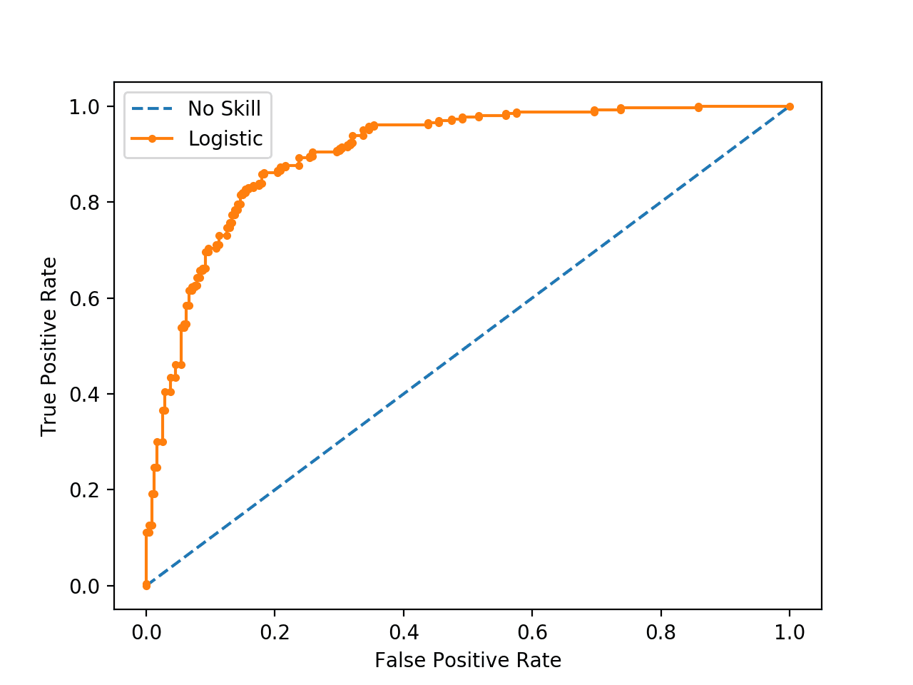
ROC Curve Plot for a No Skill Classifier and a Logistic Regression Model

What Are Precision-Remember Curves?

There are many means to evaluate the skill of a prediction model.

An arroyo in the related field of information retrieval (finding documents based on queries) measures precision and recall.

These measures are as well useful in applied automobile learning for evaluating binary classification models.

Precision is a ratio of the number of true positives divided by the sum of the truthful positives and false positives. It describes how skillful a model is at predicting the positive class. Precision is referred to as the positive predictive value.

Positive Predictive Ability = True Positives / (Truthful Positives + False Positives)

or

Precision = Truthful Positives / (True Positives + Imitation Positives)

Recollect is calculated equally the ratio of the number of true positives divided by the sum of the true positives and the false negatives. Retrieve is the aforementioned as sensitivity.

Recall = True Positives / (True Positives + False Negatives)

or

Sensitivity = Truthful Positives / (True Positives + False Negatives)

Reviewing both precision and recall is useful in cases where there is an imbalance in the observations between the ii classes. Specifically, there are many examples of no event (grade 0) and only a few examples of an event (class i).

The reason for this is that typically the large number of class 0 examples means we are less interested in the skill of the model at predicting form 0 correctly, e.g. high true negatives.

Key to the calculation of precision and recollect is that the calculations do not brand use of the true negatives. It is only concerned with the correct prediction of the minority class, class ane.

A precision-retrieve bend is a plot of the precision (y-axis) and the recall (x-axis) for different thresholds, much similar the ROC curve.

A no-skill classifier is one that cannot discriminate betwixt the classes and would predict a random class or a constant class in all cases. The no-skill line changes based on the distribution of the positive to negative classes. It is a horizontal line with the value of the ratio of positive cases in the dataset. For a balanced dataset, this is 0.five.

While the baseline is fixed with ROC, the baseline of [precision-recall curve] is determined by the ratio of positives (P) and negatives (N) as y = P / (P + North). For instance, we accept y = 0.v for a balanced course distribution …

— The Precision-Remember Plot Is More Informative than the ROC Plot When Evaluating Binary Classifiers on Imbalanced Datasets, 2022.

A model with perfect skill is depicted as a point at (1,1). A skilful model is represented past a curve that bows towards (i,ane) above the flat line of no skill.

There are as well composite scores that attempt to summarize the precision and call back; two examples include:

• F-Measure or F1 score: that calculates the harmonic mean of the precision and recall (harmonic hateful because the precision and call back are rates).
• Expanse Nether Bend: like the AUC, summarizes the integral or an approximation of the expanse under the precision-call back curve.

In terms of model selection, F-Mensurate summarizes model skill for a specific probability threshold (eastward.g. 0.v), whereas the surface area nether curve summarize the skill of a model beyond thresholds, like ROC AUC.

This makes precision-retrieve and a plot of precision vs. think and summary measures useful tools for binary classification issues that have an imbalance in the observations for each class.

Precision-Remember Curves in Python

Precision and recall can be calculated in scikit-acquire.

The precision and call back tin be calculated for thresholds using the precision_recall_curve() part that takes the true output values and the probabilities for the positive class as input and returns the precision, recall and threshold values.

. . . # summate precision-retrieve bend precision , recall , thresholds = precision_recall_curve ( testy , probs )

The F-Measure out tin can be calculated by calling the f1_score() office that takes the true form values and the predicted grade values as arguments.

. . . # calculate F1 score f1 = f1_score ( testy , yhat )

The area under the precision-recall curve tin be approximated by calling the auc() office and passing it the recall (x) and precision (y) values calculated for each threshold.

. . . # calculate precision-recollect AUC auc = auc ( recall , precision )

When plotting precision and recall for each threshold as a curve, it is of import that call up is provided equally the x-axis and precision is provided every bit the y-axis.

The consummate example of calculating precision-call back curves for a Logistic Regression model is listed below.

1 2 iii 4 5 6 7 8 9 10 11 12 thirteen xiv 15 16 17 18 xix 20 21 22 23 24 25 26 27 28 29 30 31 32 33 34 35 36

# precision-recall curve and f1 from sklearn . datasets import make_classification from sklearn . linear_model import LogisticRegression from sklearn . model_selection import train_test_split from sklearn . metrics import precision_recall_curve from sklearn . metrics import f1_score from sklearn . metrics import auc from matplotlib import pyplot # generate ii form dataset X , y = make_classification ( n_samples = 1000 , n_classes = 2 , random_state = ane ) # split into train/test sets trainX , testX , trainy , testy = train_test_split ( X , y , test_size = 0.5 , random_state = 2 ) # fit a model model = LogisticRegression ( solver = 'lbfgs' ) model . fit ( trainX , trainy ) # predict probabilities lr_probs = model . predict_proba ( testX ) # keep probabilities for the positive effect just lr_probs = lr_probs [ : , one ] # predict class values yhat = model . predict ( testX ) lr_precision , lr_recall , _ = precision_recall_curve ( testy , lr_probs ) lr_f1 , lr_auc = f1_score ( testy , yhat ) , auc ( lr_recall , lr_precision ) # summarize scores print ( 'Logistic: f1=%.3f auc=%.3f' % ( lr_f1 , lr_auc ) ) # plot the precision-recall curves no_skill = len ( testy [ testy == 1 ] ) / len ( testy ) pyplot . plot ( [ 0 , 1 ] , [ no_skill , no_skill ] , linestyle = '--' , characterization = 'No Skill' ) pyplot . plot ( lr_recall , lr_precision , marker = '.' , label = 'Logistic' ) # axis labels pyplot . xlabel ( 'Recall' ) pyplot . ylabel ( 'Precision' ) # bear witness the legend pyplot . legend ( ) # show the plot pyplot . evidence ( )

Running the instance first prints the F1, surface area nether curve (AUC) for the logistic regression model.

Note: Your results may vary given the stochastic nature of the algorithm or evaluation procedure, or differences in numerical precision. Consider running the example a few times and compare the boilerplate outcome.

Logistic: f1=0.841 auc=0.898

The precision-think bend plot is and then created showing the precision/call back for each threshold for a logistic regression model (orangish) compared to a no skill model (blueish).

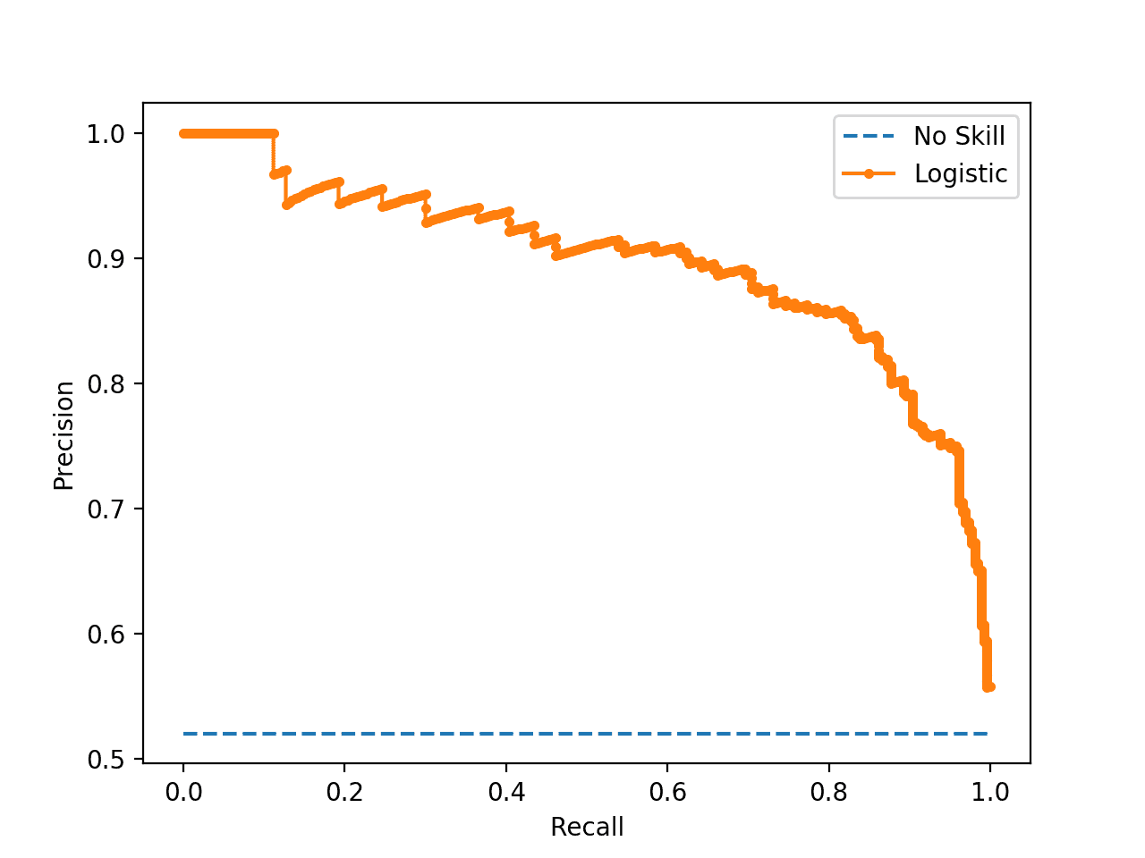
Precision-Retrieve Plot for a No Skill Classifier and a Logistic Regression Model

When to Use ROC vs. Precision-Remember Curves?

More often than not, the use of ROC curves and precision-retrieve curves are every bit follows:

• ROC curves should exist used when there are roughly equal numbers of observations for each class.
• Precision-Recollect curves should exist used when there is a moderate to large class imbalance.

The reason for this recommendation is that ROC curves nowadays an optimistic picture of the model on datasets with a class imbalance.

However, ROC curves can present an overly optimistic view of an algorithm's operation if there is a large skew in the class distribution. […] Precision-Recall (PR) curves, ofttimes used in Information Retrieval , have been cited equally an culling to ROC curves for tasks with a large skew in the class distribution.

— The Relationship Between Precision-Recall and ROC Curves, 2006.

Some become further and propose that using a ROC curve with an imbalanced dataset might be deceptive and lead to wrong interpretations of the model skill.

[…] the visual interpretability of ROC plots in the context of imbalanced datasets can exist deceptive with respect to conclusions well-nigh the reliability of nomenclature performance, attributable to an intuitive simply wrong interpretation of specificity. [Precision-think curve] plots, on the other hand, can provide the viewer with an accurate prediction of future classification performance due to the fact that they evaluate the fraction of true positives amidst positive predictions

— The Precision-Recall Plot Is More Informative than the ROC Plot When Evaluating Binary Classifiers on Imbalanced Datasets, 2022.

The chief reason for this optimistic picture is considering of the use of true negatives in the False Positive Charge per unit in the ROC Curve and the careful abstention of this rate in the Precision-Recollect bend.

If the proportion of positive to negative instances changes in a test set up, the ROC curves will not modify. Metrics such equally accuracy, precision, elevator and F scores employ values from both columns of the defoliation matrix. As a class distribution changes these measures volition alter as well, even if the fundamental classifier performance does not. ROC graphs are based upon TP rate and FP rate, in which each dimension is a strict columnar ratio, so practise not depend on class distributions.

— ROC Graphs: Notes and Applied Considerations for Data Mining Researchers, 2003.

We can make this concrete with a short example.

Beneath is the same ROC Curve instance with a modified problem where there is a ratio of nigh 100:1 ratio of class=0 to class=1 observations (specifically Class0=985, Class1=15).

i two iii four 5 6 7 8 9 x 11 12 thirteen 14 xv xvi 17 eighteen 19 twenty 21 22 23 24 25 26 27 28 29 30 31 32 33 34 35 36 37 38 39

# roc curve and auc on an imbalanced dataset from sklearn . datasets import make_classification from sklearn . linear_model import LogisticRegression from sklearn . model_selection import train_test_split from sklearn . metrics import roc_curve from sklearn . metrics import roc_auc_score from matplotlib import pyplot # generate two grade dataset Ten , y = make_classification ( n_samples = 1000 , n_classes = 2 , weights = [ 0.99 , 0.01 ] , random_state = 1 ) # split into train/test sets trainX , testX , trainy , testy = train_test_split ( Ten , y , test_size = 0.5 , random_state = 2 ) # generate a no skill prediction (majority class) ns_probs = [ 0 for _ in range ( len ( testy ) ) ] # fit a model model = LogisticRegression ( solver = 'lbfgs' ) model . fit ( trainX , trainy ) # predict probabilities lr_probs = model . predict_proba ( testX ) # keep probabilities for the positive outcome only lr_probs = lr_probs [ : , 1 ] # calculate scores ns_auc = roc_auc_score ( testy , ns_probs ) lr_auc = roc_auc_score ( testy , lr_probs ) # summarize scores print ( 'No Skill: ROC AUC=%.3f' % ( ns_auc ) ) print ( 'Logistic: ROC AUC=%.3f' % ( lr_auc ) ) # calculate roc curves ns_fpr , ns_tpr , _ = roc_curve ( testy , ns_probs ) lr_fpr , lr_tpr , _ = roc_curve ( testy , lr_probs ) # plot the roc bend for the model pyplot . plot ( ns_fpr , ns_tpr , linestyle = '--' , characterization = 'No Skill' ) pyplot . plot ( lr_fpr , lr_tpr , marker = '.' , label = 'Logistic' ) # axis labels pyplot . xlabel ( 'False Positive Rate' ) pyplot . ylabel ( 'True Positive Charge per unit' ) # show the legend pyplot . fable ( ) # show the plot pyplot . show ( )

Running the case suggests that the model has skill.

Annotation: Your results may vary given the stochastic nature of the algorithm or evaluation procedure, or differences in numerical precision. Consider running the example a few times and compare the average outcome.

No Skill: ROC AUC=0.500 Logistic: ROC AUC=0.716

Indeed, it has skill, but all of that skill is measured every bit making correct true negative predictions and there are a lot of negative predictions to make.

If you lot review the predictions, you will run into that the model predicts the majority class (class 0) in all cases on the test set. The score is very misleading.

A plot of the ROC Bend confirms the AUC interpretation of a skilful model for most probability thresholds.

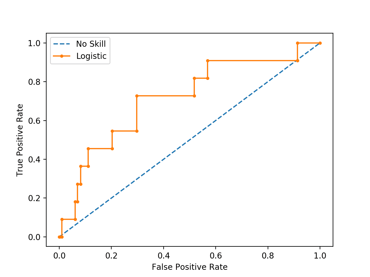
ROC Curve Plot for a No Skill Classifier and a Logistic Regression Model for an Imbalanced Dataset

Nosotros tin can too repeat the test of the same model on the aforementioned dataset and calculate a precision-recall curve and statistics instead.

The complete example is listed beneath.

one ii 3 four 5 6 7 viii 9 10 11 12 thirteen fourteen 15 sixteen 17 18 19 20 21 22 23 24 25 26 27 28 29 30 31 32 33 34 35 36 37 38

# precision-recall curve and f1 for an imbalanced dataset from sklearn . datasets import make_classification from sklearn . linear_model import LogisticRegression from sklearn . model_selection import train_test_split from sklearn . metrics import precision_recall_curve from sklearn . metrics import f1_score from sklearn . metrics import auc from matplotlib import pyplot # generate ii class dataset X , y = make_classification ( n_samples = 1000 , n_classes = 2 , weights = [ 0.99 , 0.01 ] , random_state = 1 ) # split into railroad train/examination sets trainX , testX , trainy , testy = train_test_split ( 10 , y , test_size = 0.five , random_state = two ) # fit a model model = LogisticRegression ( solver = 'lbfgs' ) model . fit ( trainX , trainy ) # predict probabilities lr_probs = model . predict_proba ( testX ) # proceed probabilities for the positive outcome simply lr_probs = lr_probs [ : , 1 ] # predict course values yhat = model . predict ( testX ) # calculate precision and call up for each threshold lr_precision , lr_recall , _ = precision_recall_curve ( testy , lr_probs ) # calculate scores lr_f1 , lr_auc = f1_score ( testy , yhat ) , auc ( lr_recall , lr_precision ) # summarize scores print ( 'Logistic: f1=%.3f auc=%.3f' % ( lr_f1 , lr_auc ) ) # plot the precision-recall curves no_skill = len ( testy [ testy == 1 ] ) / len ( testy ) pyplot . plot ( [ 0 , 1 ] , [ no_skill , no_skill ] , linestyle = '--' , label = 'No Skill' ) pyplot . plot ( lr_recall , lr_precision , marking = '.' , label = 'Logistic' ) # axis labels pyplot . xlabel ( 'Recollect' ) pyplot . ylabel ( 'Precision' ) # prove the legend pyplot . fable ( ) # testify the plot pyplot . show ( )

Running the instance start prints the F1 and AUC scores.

Note: Your results may vary given the stochastic nature of the algorithm or evaluation process, or differences in numerical precision. Consider running the instance a few times and compare the average outcome.

Nosotros can see that the model is penalized for predicting the bulk grade in all cases. The scores show that the model that looked good co-ordinate to the ROC Curve is in fact barely good when considered using using precision and recall that focus on the positive class.

Logistic: f1=0.000 auc=0.054

The plot of the precision-recall curve highlights that the model is only barely above the no skill line for most thresholds.

This is possible because the model predicts probabilities and is uncertain about some cases. These get exposed through the different thresholds evaluated in the construction of the curve, flipping some class 0 to class 1, offering some precision but very depression recall.

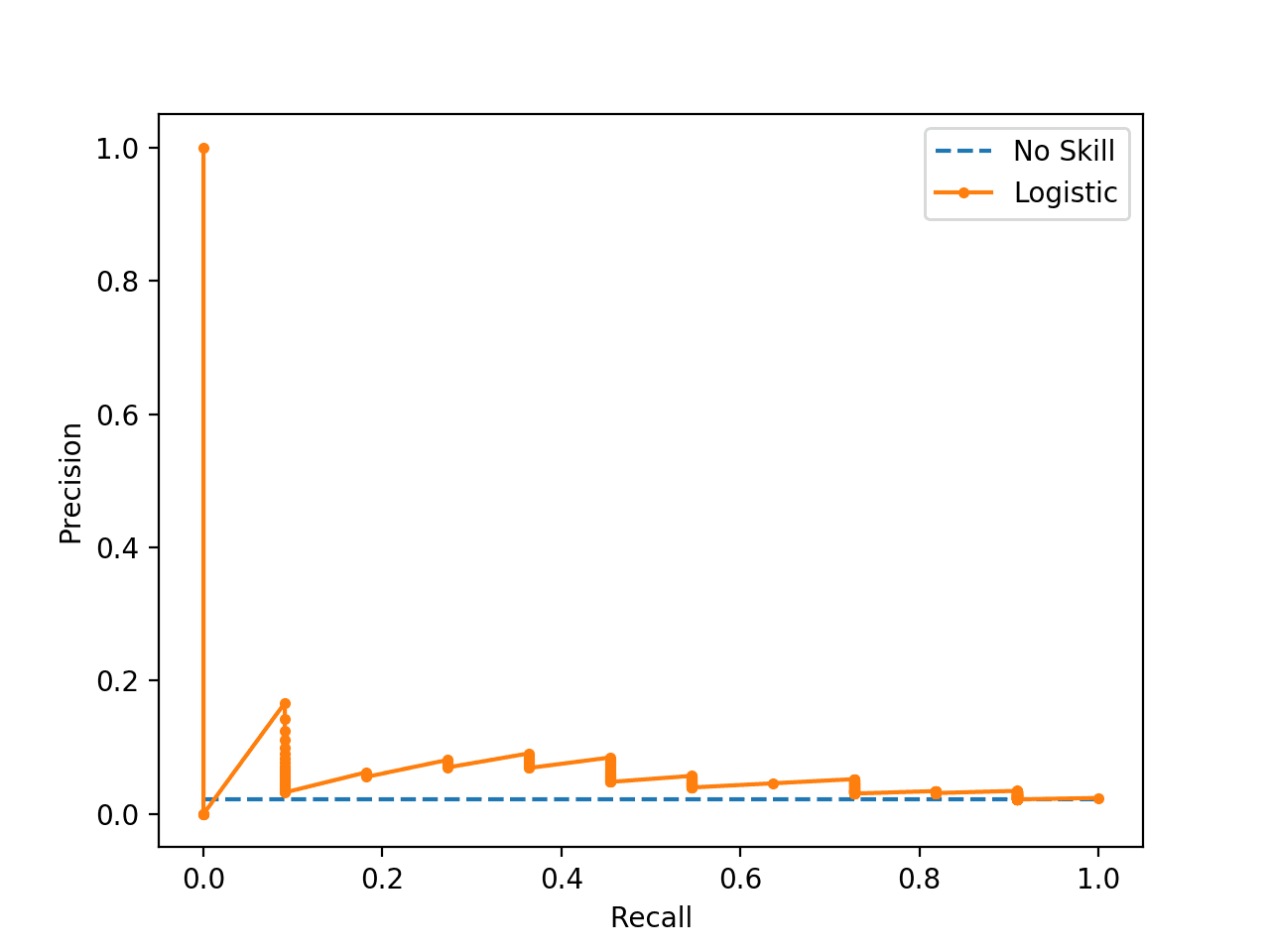
Precision-Recall Plot for a No Skill Classifier and a Logistic Regression Model for am Imbalanced Dataset

Further Reading

This section provides more resources on the topic if you are looking to go deeper.

Papers

• A disquisitional investigation of call up and precision equally measures of retrieval system operation, 1989.
• The Relationship Betwixt Precision-Recall and ROC Curves, 2006.
• The Precision-Recall Plot Is More Informative than the ROC Plot When Evaluating Binary Classifiers on Imbalanced Datasets, 2022.
• ROC Graphs: Notes and Practical Considerations for Information Mining Researchers, 2003.

API

• sklearn.metrics.roc_curve API
• sklearn.metrics.roc_auc_score API
• sklearn.metrics.precision_recall_curve API
• sklearn.metrics.auc API
• sklearn.metrics.average_precision_score API
• Precision-Recall, scikit-larn
• Precision, think and F-measures, scikit-larn

Articles

• Receiver operating characteristic on Wikipedia
• Sensitivity and specificity on Wikipedia
• Precision and recall on Wikipedia
• Information retrieval on Wikipedia
• F1 score on Wikipedia
• ROC and precision-recall with imbalanced datasets, blog.

Summary

In this tutorial, you discovered ROC Curves, Precision-Think Curves, and when to employ each to interpret the prediction of probabilities for binary classification problems.

Specifically, you learned:

• ROC Curves summarize the trade-off between the true positive rate and false positive rate for a predictive model using different probability thresholds.
• Precision-Recall curves summarize the trade-off between the truthful positive charge per unit and the positive predictive value for a predictive model using unlike probability thresholds.
• ROC curves are appropriate when the observations are counterbalanced between each class, whereas precision-recall curves are advisable for imbalanced datasets.

Do you have whatsoever questions?
Ask your questions in the comments below and I will practise my all-time to answer.

Get a Handle on Probability for Machine Learning!

Develop Your Agreement of Probability

...with simply a few lines of python code

Discover how in my new Ebook:
Probability for Machine Learning

It provides self-study tutorials and stop-to-end projects on:
Bayes Theorem, Bayesian Optimization, Distributions, Maximum Likelihood, Cross-Entropy, Calibrating Models
and much more...

Finally Harness Doubt in Your Projects

Skip the Academics. Just Results.

Run across What'due south Within

Source: https://machinelearningmastery.com/roc-curves-and-precision-recall-curves-for-classification-in-python/

Posted by: tatesincom.blogspot.com

Share this post